Continuous data: normally-distributed data histogram to math normal function curve

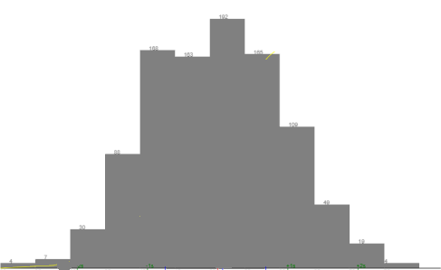
n=1000 From normal population μ=100 σ=10

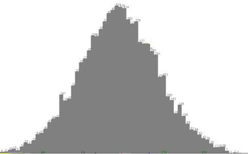
n=10000 From normal population μ=100 σ=10
class widths narrower, more of them.
Histogram here scaled to look same size as above. It has ten times the data, so is actually ten times as large, unscaled.

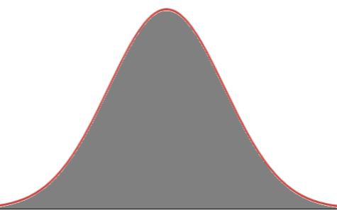
In the limit, as n gets very large, e.g. N, (actually, to ∞), class width narrows to zero and the histogram becomes smoother and smoother, we can step into a math function and its curve. And do math stuff.

ƒ(x) =		😂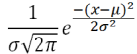

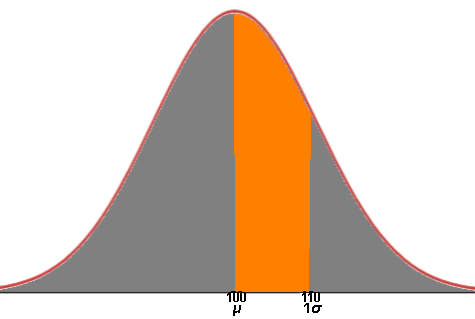
For example:

μ=100 σ=10

ƒ(x) =

(This graph has to have its Y axis greatly magnified/stretched in order to see the mound. The X and Y axes don't have to be at the same scale. Every normal curve, of whatever μ and σ, can be made to look similar to the one here.)
Unlike most math functions/curves we aren't interested in the function's y values, i.e. the points on the curve, but only in the area under the curve on intervals e.g. [95,100], or [100,110] etc.
Area under the curve equals 1, i.e. 100% of the data, 100% of the probability.
The area (a number between 0 and 1) is the probability (a number between 0 and 1) that a datum is in that interval. The precentage of the data that is in the interval.

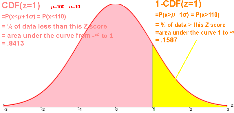
The orange is the area under the curve on the interval [100,110], which is [μ,1σ], which is an Empircal Rule "slice" of 34.1%.

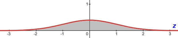
μ=0 σ=1 is the standard normal function/curve/distribution.
Its function simplifies 😉 to

ƒ(x) =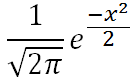

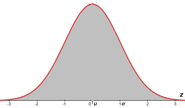
It looks naturally (unscaled) like this:
So it's typically vertically stretched to look like the above normal curves:

We can think of the horizontal axis as the Z axis and the function as a function of z:

ƒ(z) =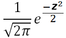

For a normal population, a Z score is the number of standard deviations (σ=1) from the mean (μ=0) of this standard normal curve.
We convert a datum to its z-score because we then find out its CDF (cumulative density function) value (the area under the curve from -∞ to this z score, which equals the percent of the population that is less than this datum, which equals the probability that a random selection from the population will be less than this datum) by either looking up the CDF in a Z table or having a calculator or software calculate it for us.